Rust Machine Learning Book

Using DBSCAN with linfa-clustering

What is the DBSCAN algorithm?

The DBSCAN algorithm (Density-Based Spatial Clustering Algorithm with Noise) was originally published in 1996, and has since become one of the most popular and well-known clustering algorithms available.

Comparison with KMeans

Before getting into the code, let's examine how these differences in approach plays out on different types of data. In the images below, both the DBSCAN and KMeans algorithms were applied to the same dataset. The KMeans algorithm was manually set to find 3 clusters (remember, DBSCAN automatically calculates the number of clusters based on the provided parameters).

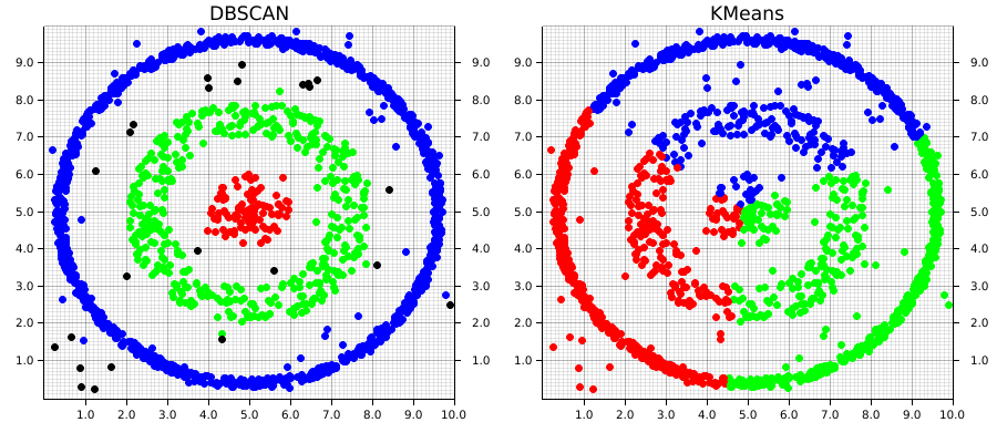
This example¹ demonstrates two of the major strengths of DBSCAN over an algorithm like KMeans; it is able to automatically detect the number of clusters that meet the set of given parameters. Keep in mind that this doesn't mean DBSCAN require less information about the dataset, but rather that the information it does require differs from an algorithm like KMeans.

DBSCAN does a great job at finding clustering that are spatially contiguous, but not necessarily confined to single region. This is where the "and Noise" part of the algorithm's name comes in. Especially in real-world data, there's often data that won't fit well into a given cluster. These can be outliers or points that don't demonstrate good alignment with any of the main clusters. DBSCAN doesn't require that they do. Instead, it will simply give them a cluster label of None (in our example, these are graphically the black points). However, DBSCAN does a good job at analyzing existing information, it doesn't predict new data, which is one of its main drawbacks

Comparatively, KMeans will take into account each point in the dataset, which means outliers can negatively affect the local optimal location for a given cluster's centroid in order to accommodate them. Euclidean space is linear, which means that small changes in the data result in proportionately small changes to the position of the centroids. This is problematic when there are outliers in the data.

Using DSBCAN with linfa

Compared to

#![allow(unused)]
fn main() {
// Import the linfa prelude and KMeans algorithm
use linfa::prelude::*;
use linfa_clustering::Dbscan;
// We'll build our dataset on our own using ndarray and rand
use ndarray::prelude::*;
// Import the plotters crate to create the scatter plot
use plotters::prelude::*;
}

Instead of having a several higher-density clusters different areas, we'll take advantage of DBSCAN's ability to follow spatially-contiguous non-localized clusters by building our data out of both filled and hollow circles, with some random noise tossed in as well. The end goal will be to re-find each of these clusters, and exclude some of the noise!

#![allow(unused)]
fn main() {
    // The goal is to be able to find each of these as distinct, and exclude some of the noise
    let circle: Array2<f32> = create_circle([5.0, 5.0], 1.0, 100); // Cluster 0
    let donut_1: Array2<f32> = create_hollow_circle([5.0, 5.0], [2.0, 3.0], 400); // Cluster 1
    let donut_2: Array2<f32> = create_hollow_circle([5.0, 5.0], [4.5, 4.75], 1000); // Cluster 2
    let noise: Array2<f32> = create_square([5.0, 5.0], 10.0, 100); // Random noise

    let data = ndarray::concatenate(
        Axis(0),
        &[circle.view(), donut_1.view(), donut_2.view(), noise.view()],
    )
    .expect("An error occurred while stacking the dataset");
}

Compared to linfa's KMeans algorithm, the DBSCAN implementation is able to operate directly on a ndarray Array2 data structure, so there's no need to convert it into the linfa-native Dataset type first. It's also worth pointing out that choosing the chosen parameters often take some experimentation and tuning before they produce results that actually make sense. This is one of the areas where data visualization can be really valuable; it is helpful in developing some spatial intuition about your data set and understand how your choice of hyperparameters will affect the results produced by the algorithm.

#![allow(unused)]
fn main() {
    // Compared to linfa's KMeans algorithm, the DBSCAN implementation can operate
    // directly on an ndarray `Array2` data structure, so there's no need to convert it
    // into the linfa-native `Dataset` first.
    let min_points = 20;
    let clusters = Dbscan::params(min_points)
        .tolerance(0.6)
        .transform(&data)
        .unwrap();
    println!("{:#?}", clusters);
}

We'll skip over setting up ChartBuilder struct and drawing areas from the plotters crate, since it's exactly the same as in the KMeans example.

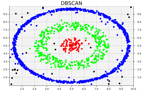
Remember how we mentioned DBSCAN is an algorithm that can exclude noise? That's particularly important for the pattern-matching in this case, since we're almost guaranteed to end up with some values that don't fit nicely into any of our expected clusters. Since we generated an artificial dataset, we know the number of clusters that should be generated, and where they're located. However, that won't always be the case. In that situation, we could instead examine the number of clusters afterwards, create a colormap using custom RGB colors which matches the highest number of clusters, and plot it that way.

#![allow(unused)]
fn main() {
    for i in 0..data.shape()[0] {
        let coordinates = data.slice(s![i, 0..2]);

        let point = match clusters[i] {
            Some(0) => Circle::new(
                (coordinates[0], coordinates[1]),
                3,
                ShapeStyle::from(&RED).filled(),
            ),
            Some(1) => Circle::new(
                (coordinates[0], coordinates[1]),
                3,
                ShapeStyle::from(&GREEN).filled(),
            ),
            Some(2) => Circle::new(
                (coordinates[0], coordinates[1]),
                3,
                ShapeStyle::from(&BLUE).filled(),
            ),
            // Making sure our pattern-matching is exhaustive
            // Note that we can define a custom color using RGB
            _ => Circle::new(
                (coordinates[0], coordinates[1]),
                3,
                ShapeStyle::from(&RGBColor(255, 255, 255)).filled(),
            ),
        };

        root_area
            .draw(&point)
            .expect("An error occurred while drawing the point!");
    }
}

As a result, we then get the following chart, where each cluster is uniquely identified, and some of the random noise associated with the dataset is discarded.